Analysis
Please, see the data preparation tutorial for understand how to prepare data for this functions.
Load data
import pandas as pd
df = pd.read_csv('example_datasets/train.csv')
First steps
In this tutorial, we will describe the onboarding lost-passed case.
Goal
Our goal is to detect interface elements/screens of an app at which users’ engagement drops significantly and induces them to leave the app without account registration.
Tasks
Collect data
Prepare data
Analyze data
Build pivot tables
Visualize users path in the app
Build the classifier
- Classifier helps you to pick out specific users paths
- Classifier allows estimating the probability of the user’s leaving from the app based on his current path. One can use this information to dynamically change the content of the app to prevent that.
Expected results
- You will identify the most “problematic” elements of the app
- You will get the classifier which will allow you to predict the user’s leaving from the app based on the current user’s behavior
Import retentioneering framework
First of all, we need to import package module
from retentioneering import analysis
After that we shoud select the export folder in config (you can leave it empty and the script will create a folder with current timestamp). Note: if you don’t want to leave this field empty, you have to specify an existing directory, because the script will not create it.
settings = {
    'export_folder': './experiments/new_experiment'
}
or
settings = {}
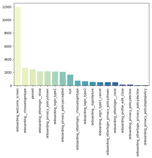
Events` probability dynamics
desc = analysis.get_desc_table(df,
                               settings=settings,
                               plot=True,
                               target_event_list=['lost',
                                                  'passed'])
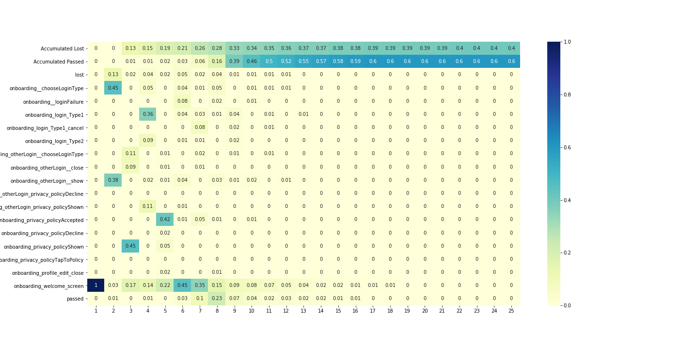
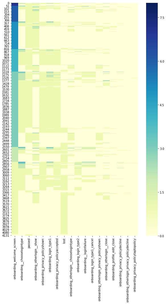
- Each column of the table corresponds to a sequence number
- of the user’s steps from the path and each row corresponds to event name.
Values of the table show the probability that the user choose the appropriate event at the appropriate step.
- It’s difficult to make a complex analysis from that table so it is better
- to split our users to those who leave the app and those who passed.
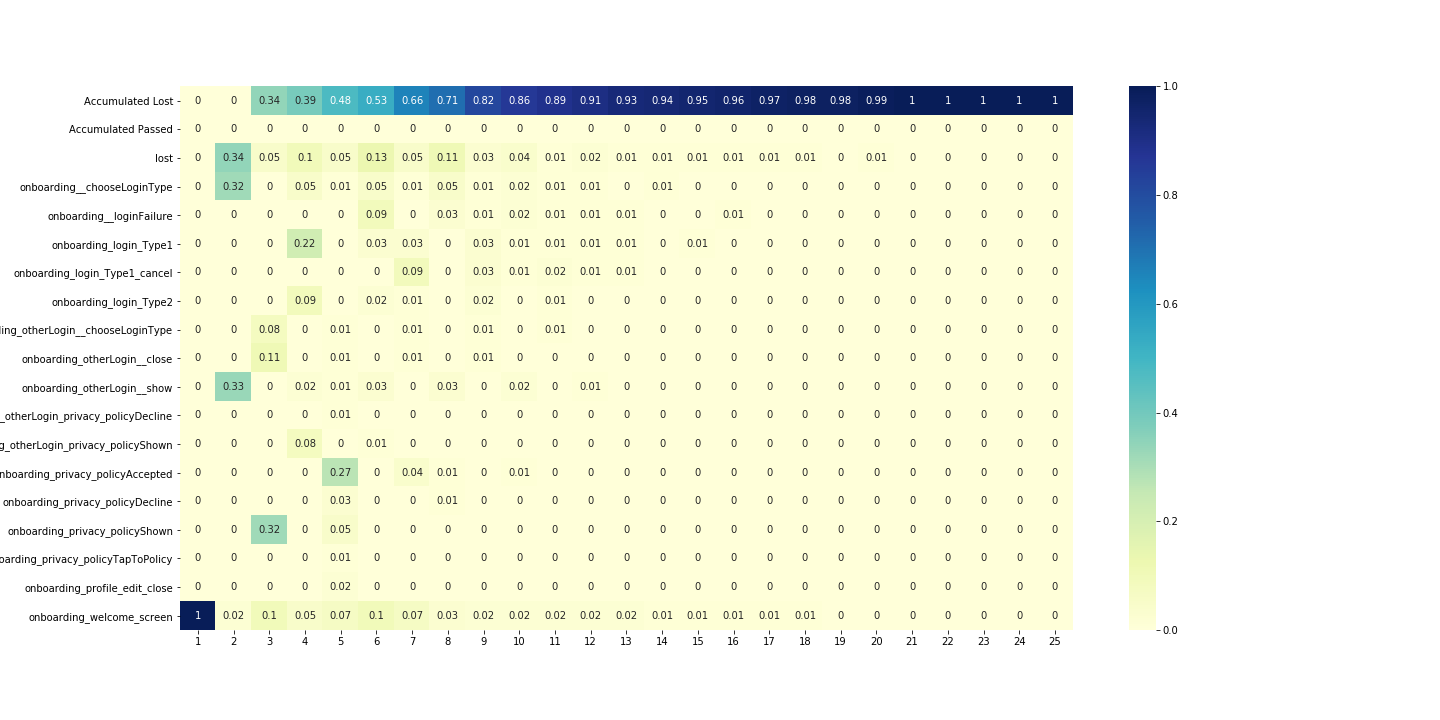
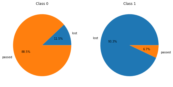
Difference in passed and lost users behaviour
# find users who get lost
lost_users_list = df[df.event_name == 'lost'].user_pseudo_id.unique()

# create filter for lost users
filt = df.user_pseudo_id.isin(lost_users_list)

# filter data for lost users trajectories
df_lost = df[filt]

# filter data for passed users trajectories
df_passed = df[~filt]
Plot dynamics for different groups.
Plot for group of users who have lost event:
desc_loss = analysis.get_desc_table(df_lost,
                                    settings=settings,
                                    plot=True,
                                    target_event_list=['lost',
                                                       'passed'])
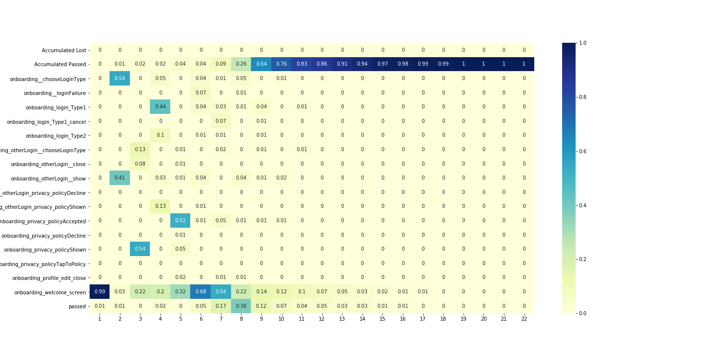
Plot for group of users who have passed event:
desc_passed = analysis.get_desc_table(df_passed,
                                    settings=settings,
                                    plot=True,
                                    target_event_list=['lost',
                                                       'passed'])
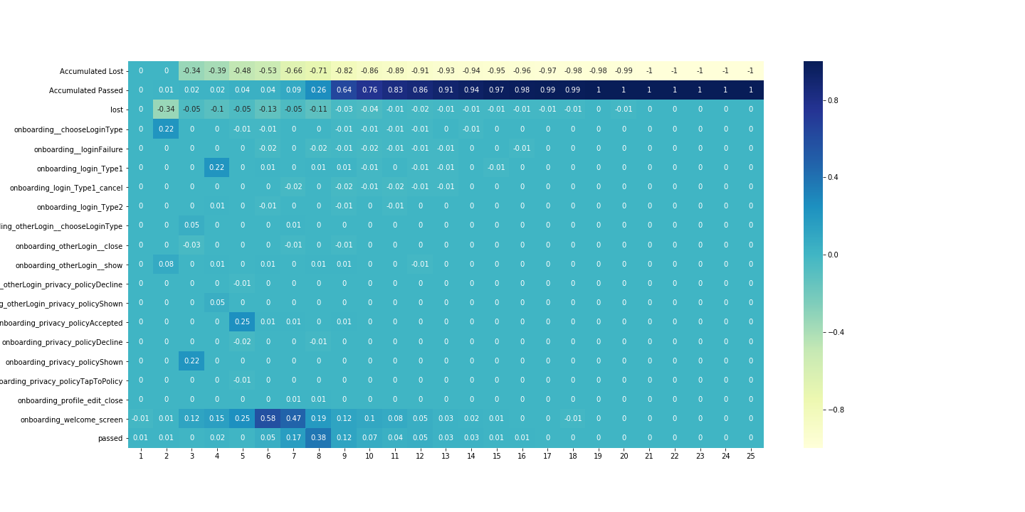
diff_df = analysis.get_diff(desc_loss,
                            desc_passed,
                            settings=settings,
                            precalc=True)
Agregates over user transitions
Lets aggregate our data over users transitions:
agg_list = ['trans_count', 'dt_mean', 'dt_median', 'dt_min', 'dt_max']
df_agg = analysis.get_all_agg(df, agg_list)
df_agg.head()
Out:
                    event_name                      next_event  trans_count    ...
0  onboarding__chooseLoginType                            lost            1    ...
1  onboarding__chooseLoginType          onboarding_login_Type1          414    ...
2  onboarding__chooseLoginType          onboarding_login_Type2          159    ...
3  onboarding__chooseLoginType  onboarding_privacy_policyShown         2133    ...
4     onboarding__loginFailure                            lost            1    ...
Now we can see which transitions take the most time and how often people have used different transitions.
We could choose the 10 longest users’ paths:
df_agg.sort_values('trans_count', ascending=False).head(10)
Out:
                           event_name                         next_event  trans_count    ...
84          onboarding_welcome_screen          onboarding_welcome_screen         5021    ...
85          onboarding_welcome_screen                             passed         2330    ...
3         onboarding__chooseLoginType     onboarding_privacy_policyShown         2133    ...
79          onboarding_welcome_screen        onboarding__chooseLoginType         1938    ...
67     onboarding_privacy_policyShown             onboarding_login_Type1         1675    ...
11             onboarding_login_Type1  onboarding_privacy_policyAccepted         1666    ...
82          onboarding_welcome_screen        onboarding_otherLogin__show         1601    ...
62  onboarding_privacy_policyAccepted          onboarding_welcome_screen         1189    ...
78          onboarding_welcome_screen                               lost         1043    ...
47        onboarding_otherLogin__show          onboarding_welcome_screen          876    ...
You can see the events where users spend most of their time. It seems reasonable to analyze only popular events to get stable results.
Adjacency matrix
The adjacency matrix is the representation of the graph. You can read more about it on the`wiki <https://en.wikipedia.org/wiki/Adjacency_matrix>`__:
adj_count = analysis.get_adjacency(df_agg, 'trans_count')
adj_count
Out:
                                        ...   onboarding_login_Type1   onboarding_privacy_policyShown    ...
onboarding_login_Type1                  ...                      0.0                              0.0    ...
onboarding_privacy_policyShown          ...                   1675.0                              0.0    ...
onboarding__loginFailure                ...                      0.0                              0.0    ...
onboarding_privacy_policyTapToPolicy    ...                      0.0                              0.0    ...
onboarding_welcome_screen               ...                      0.0                              0.0    ...
Users clustering
Also, we could clusterize users by the frequency of events in their path:
countmap = analysis.calculate.calculate_frequency_map(df, settings)
On that plot, we can see that some users have pretty close frequencies of different functions usage.
And we can see that it is useful to separate groups with different conversion rates:
analysis.utils.plot_clusters(df, countmap, n_clusters=5, plot_cnt=2)
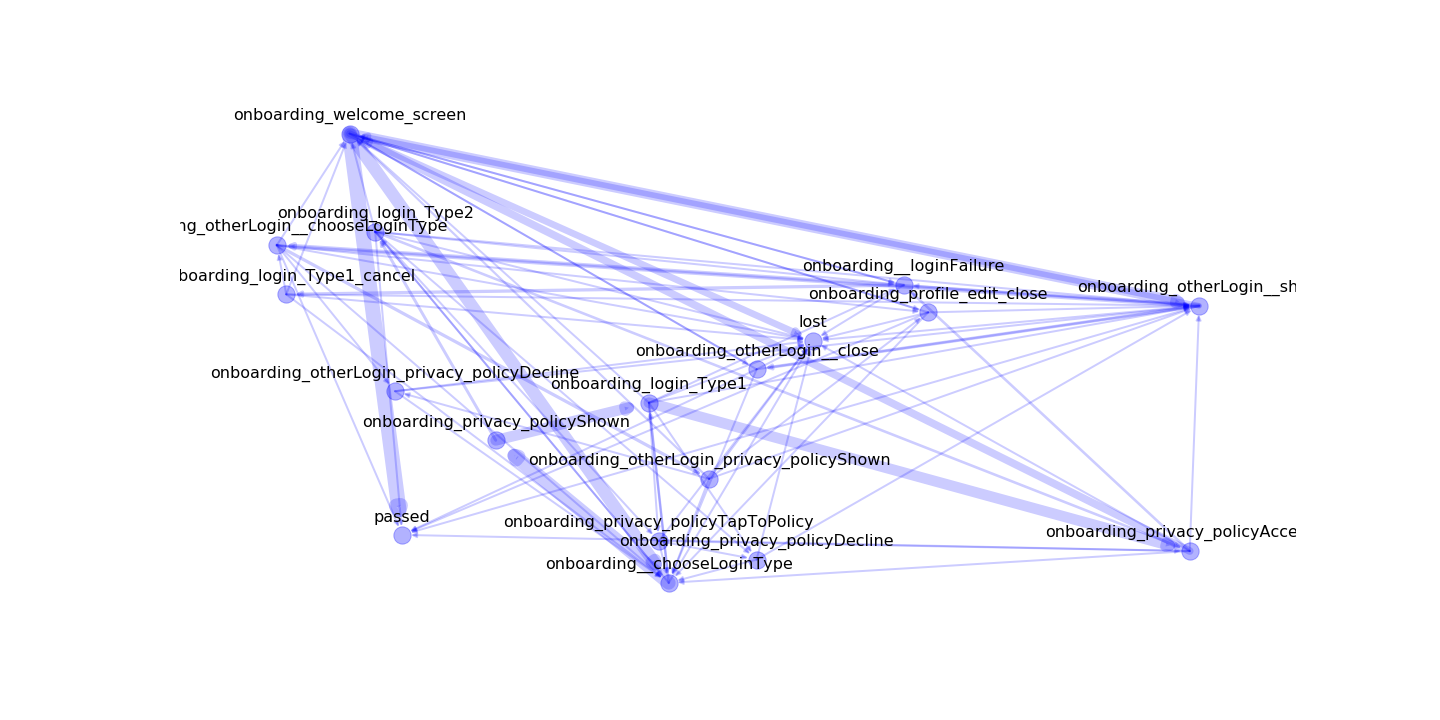
Graph visualization
We have two options to plot the graphs:
1. With python (this is local)
2. With our API
(in that case, you'll send your data to our servers, but we don't save it and using only for visualization)
In the second option, the plot looks much better and obvious.
analysis.utils.plot_graph_python(df_agg, 'trans_count', settings)
from retentioneering.utils.export import plot_graph_api
plot_graph_api(df_lost, settings)
Lost-Passed classifier
Model fitting
clf = analysis.Model(df, target_event='lost', settings=settings)
clf.fit_model()
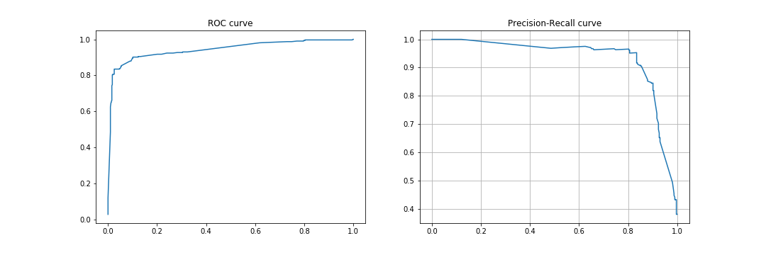
It returns metrics of quality of the model.
Model inference
We have data for new users, who are not passed or lost already.
Lets load it into pandas DataFrame:
test_data = pd.read_csv('example_datasets/test.csv')
Now we can predict probabilities for new users:
prediction = clf.infer(test_data)
prediction.head()
Out:
                     user_pseudo_id  not_target    target
0  000bf8e1812a0335c7e65d52b3f6e816    0.976125  0.023875
1  00275391998b3f87d798f6e7a1ec5c15    0.757970  0.242030
2  004ecbe8a710f3c7b5b3cbc9bc0c74b2    0.727521  0.272479
3  00530441b09d5494b09e936a97d5cb99    0.988654  0.011346
4  005502038cec478faf343fe54310a848    0.592515  0.407485
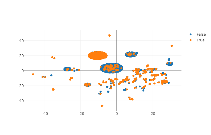
Understanding your data
You can plot projection of users trajectories to understand how your data looks likes:
clf.plot_projections()
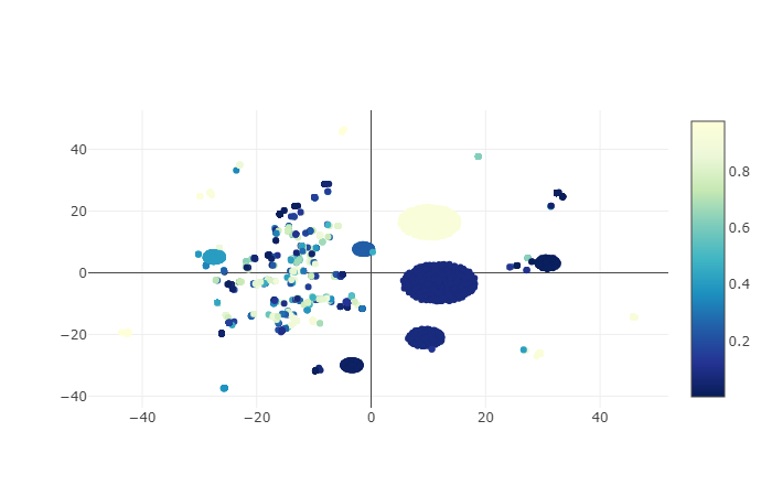
Understanding prediction of your model
Also, you can plot results of the model inference over that projections to understand the cases where your model fails:
clf.plot_projections(sample=data.event_name.values, ids=data.user_pseudo_id.values)
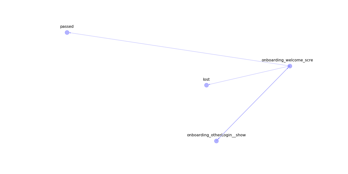
Visualizing graph for area
From the previous plot, you can be interested in what trajectories has high conversion rates.
You can select the area on that plot and visualize it as a graph:
# write coordinates bbox angles

bbox = [
    [-4, -12],
    [8, -26]
]

clf.plot_cluster_track(bbox)
The most important edges
You could find what was the most important edges and nodes in your model for debugging (e.g. it helps you to understand ‘leaky’ events) or to find problem transitions in your app.
Edges:
imp_tracks = clf.build_important_track()
imp_tracks[imp_tracks[1].notnull()]
Out:
                             0                              1
0  onboarding__chooselogintype         onboarding_login_type1
1       onboarding_login_type1       onboarding__loginfailure
2  onboarding__chooselogintype         onboarding_login_type2
3       onboarding_login_type2    onboarding_otherlogin__show
5     onboarding__loginfailure  onboarding_login_type1_cancel
Nodes:
imp_tracks[imp_tracks[1].isnull()][0].values
Out:
array(['onboarding__loginfailure', 'onboarding_login_type1',
       'onboarding_login_type1_cancel', 'onboarding_login_type2',
       'onboarding_otherlogin_privacy_policyshown',
       'onboarding_privacy_policydecline', 'onboarding_welcome_screen'],
      dtype=object)